Mathematical Functions in Excel

Excel Tutorial 03: Mathematical Functions in Excel

We will be dealing with MIN, MAX, RAND, ROUND, POWER functions in this release.

So, let's get started

1. MIN: This function is used to find the minimum number among the range of selected cells, it does not take into consideration the logical value and text.

Syntax: MIN(number1,.....)

number1: Is the range of selected cells among which the maximum is to be searched

Output: Minimum value of the selected range of cells

Example:

Note: You can use MINA for taking into consideration logical value and text and MINIFS for conditional based calculation

2. MAX: This function is used to find the maximum number among the range of selected cells, it does not take into consideration the logical value and text.

Syntax: MAX(number1,.....)

number1: Is the range of selected cells among which the maximum is to be searched

Output: Maximum value of the selected range of cells

Example:

Note: You can use MAXA for taking into consideration logical value and text and MAXIFS for conditional based calculation

3. RAND: This function is used as a random number generator in excel. It takes no argument and produces values between 0 and 1.

Syntax: RAND()

Output: Random number between 0 and 1

Example:

Here we can see 5 random number generated using it and which can further be multiplied by 10 and then using the ROUND function can be used to generate 5 random integers

4. ROUND: This function is used to round up decimal numbers with x precision to a particular precision of n digits, what it effectively does is it takes the decimal and omits any digits after the x number of digits to the right of the decimal point

Syntax: ROUND(number,num_digits)

number: Is the number or the decimal
num_digits: Is the precision

Output: Decimal rounded to x precision

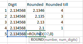
Example:

Here we can see the decimal 2.1346 is rounded to a different level of precision

5. POWER: This function is used to find the exponential output of any number N raised to the power of x

Syntax: POWER(number,power)

number: Is the number or the base
power: Is the power / the multiplier to which the base is raised

Output: Power value of N raised to x

Example:

Here we can see we are finding the 2 raised to the power of various values

We will try to cover some more useful functions like match, find, vlookup, index, etc in the next tutorial and soon will start with formulae related to text like left, mid, right, trim, etc.

Excel Tutorial 02: Arithmetic Functions Continued in Excel

Excel Tutorial 02: Arithmetic Functions Continued in Excel

We will be dealing with the various variants of the SUM, COUNT, AVERAGE function in this release.

So, let's get started

1. SUM:

• SUMIF: It is used to return the addition of a selected range of cells on the basis of a condition, i.e it only adds those cell which actually satisfies the condition.

         The condition supports the logical operation and also partial matching, the logical operation includes (>,<,<>,=) and partial matching (*,?).

         Syntax: SUMIF(range,criteria,sum_range)

         range: Is the range of cells where you want to apply conditions
         criteria: Is the condition, logical or partial matching
         sum_range: Is the range of cells of which you want the sum

Note: SUMIF is used for one condition only, you can always use SUMIFS in place of SUMIF

         Here is a capture of the example, which itself is self-explanatory

• SUMIFS: It is used to return the addition of a selected range of cells on the basis of a condition, i.e it only adds those cell which actually satisfies the condition.

         The condition supports the logical operation and also partial matching, the logical operation includes (>,<,<>,=) and partial matching (*,?).

Syntax: SUMIFS(sum_range,criteria_range1,criteria1,
criteria_range2,criteria2,.....criteria_rangeN,criteriaN)

sum_range: Is the range of cells of which you want the sum
criteria1: Is the condition, logical or partial matching
criteria_range1: Is the range of cells where you want to apply condition

Note: Here you can apply multiple conditions on multiple ranges to output the sum, it's just like many SUMIF.

Here is a capture of the example, which itself is self-explanatory

2. COUNT:

• COUNTA: It is used to count a range of selected cells, which can be chosen for multiple ranges, irrespective of the data in the cells. It counts the number of cells in those multiple cells except blank cells.

Note: How is it different from COUNT: COUNT can only count numbers and dates whereas counta can count data types of any type except blank. For blank use countblank.

Syntax: COUNTA(range1,range2,.....rangeN)

range1: Selection of multiple cells

Output: Total number of cells that are not blank

Note: COUNTA means to count all

• COUNTIF: It is used to count a selected range of cells on the basis of a condition, the condition is a logical condition.

          Syntax: countif(range,criteria)

          range: The selected range of cells which you want to count on the basis of the criteria

          criteria: Is the condition that you want to apply to count only the relevant cells

          Output: Count of the number of cells or value matching the condition

• COUNTIFS: It is used to count multiple selected range of cells on the basis of corresponding multiple conditions, the conditions are a logical condition.


Syntax: countifs(range1,criteria1,range2,criteria2,.....)


range: The selected range of cells which you want to count on the basis of the criteria
criteria: Is the condition that you want to apply to count only the relevant cells


Output: Count of the number of cells or value matching the condition

3. AVERAGE:

• AVERAGEA: It is used to average all the selection of cells, irrespective of the values, whether it is a text or a logical value. It takes true as 1 and false as 0.

Note: Average skips logical values and does not count them in calculating the average

Syntax: AVERAGEA(value1,value2....)

value1: the selection of cells whose average is to be calculated

Output: Average of the selected cells including logical values and text in the calculations too

Here is an example of how to use the function:

• AVERAGEIF: It is used to calculate the average of the selected range of cells on the basis of a condition, here the condition can be a logical or partial matching condition just like countif and sumif. 

Syntax: AVERAGEIF(range,critetia)

range: the selection of the cells of which average is to be calculated

criteria: Is the condition to apply on the range to filter the values and average only those satisfying the condition

Output: Average of the selected cells satisfying the criteria

Here is an example of how to use the function:

• AVERAGEIFS: It is used to calculate the average of the selected range of cells on the basis of multiple conditions, here the condition can be a logical or partial matching condition just like countifs and sumifs. 

Syntax: AVERAGEIFS(average_range,criteria_range1,criteria1,.........)

average_range: Selection of the cells of whose the average is to be calculated

criteria_range1: Is the selection of the cells on which the conditions are applied

criteria1: It is the criteria on the basis of which average is found out of the cells qualifying the condition/criteria.

Output: Average of the selected cells satisfying the criteria

Here is an example of how to use the function:

We have completed the basic of the arithmetic functions in Excel, we will now move into discussing more of excel formula in the next release. All of these formulae will be very important to carry out various tasks in Excel, few of them are MIN, MAX, RAND, ROUND, POWER, etc.